
Manual data layout transformation: Packed AoS vs SoA
Published:
Abstract
The packed data layout representation discussed here is inspired from the Gibbon compiler 1. The Gibbon compiler generates serialized representations of tree-like recursive data structures and generates traversals over that data by fixing a particular serialization order. The traversals are more efficient because of enhanced spatial locality. The current compiler generates a representation that serializes the data in one big buffer, we term this an AoS representation. An analogue to this would be an SoA representation with separate buffers for different fields. The source code for this experiment is available.
Overview to the Gibbon compiler
Gibbon 1 is a tree traversal accelerator that optimizes the performance of tree traversals over tree-like data. The programmer can write programs in a subset of Haskell. This high level code is then lowered to various IRs. The first level of IR involves passes that monomorphize and flatten the control flow of the program among others. The IR is put in ANF form. The second level of IR called LOCAL 2, has location information throughout the code that’s derived from a constraint system to figure out the exact positioning of tags and fields in the final destination memory region. The third level of the IR removes all the types and uses a Cursor (char*) for traversing any data type. The final level of the IR is similar to an imperative language like C. This follows code generation to C. For detailed information check out 1, 2, 3 and 4. Note that a packed layout is different from a pointer based layout. In the packed layout each Cons cell is unboxed and they are contigously allocated. However, in the pointer based layout, each Cons cell is allocated using malloc and different Cells may reside at non contiguous random memory addresses. Two Cons cells are joined in a linked list fashion. That is, the predecessor Cons cell stores the memory address of the successor Cons cell. The latter exhibits low spatial locality.
Introduction
Consider the data type definition of a Cons list in Haskell.
data List = Cons Int (List) | Nil
Throughout this blog, we will look at the data representation from the lens of the Haskell Cons list. To visualize the data representation that the Gibbon compiler generates, we can use a char for the Cons tag (1 byte) and a C int type (4 bytes) for the Integer. We can use a Cursor (char* in C) to represent a particular position in the memory for the List.
The figure below on the left shows a Cons style list in the AoS form. In this form the complete datatype is laid out in one contiguous buffer. On the right, we show the representation of the Cons style list in the SoA form. In the SoA form, the data constructors and integers are in two separate buffers. 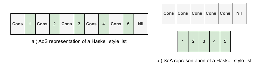
The Gibbon compiler generates a memory representation of the list similar to the one shown on the left (The AoS form). The representation on the right (SoA form) is where we would eventually want to get to.
The following delves in depth into the C code for the AoS form. In C the types look like the following.
  typedef CursorTy char*;
  typedef IntTy int;
  typedef TagTy char;
For our simple experiment, we will be allocating one big flat buffer for the AoS memory of the List. This is contrary to what Gibbon does. Gibbon uses chunk allocation to increase the allocated region by a factor of 2 every time. Gibbon starts by mallocing a small region (512 KB) by default. Then grows it dynamically. For this experiment we pre-allocate the region for simplicity reasons.
In the AoS representation where we have one big buffer, the space we need for the list can be pre-calculated as follows. Since we are using 1 byte for the Cons tag, each Cons tag takes a total of 5 bytes which includes the int. For a list size of 10,000 we need (10,000 * 5) + 1 bytes in total. This is equal to 50,001 bytes. We need 1 byte for the Nil tag. In C this look as follows:
IntTy listSize = argv[1];
CursorTy region = (CursorTy) malloc(sizeof(char) * ((5 * listSize) + 1));
Now let us look at a simple build list function in Haskell and its lowered form in C.
Haskell code:
buildList :: Int -> List
buildList len = if len <= 0
                then Nil
                else
                   let rst = buildList (len - 1)
                     in Cons len rst
The C verion of buildList looks something like this. We use a CursorTy for the memory of the List. The memory for the List is pointed to by the variable list. We return the start of the region in the variable listStart for convention. The Cons tag is represented using the character ‘0’ and the Nil tag is represented by using the character ‘1’.
Note that the C functions that we will write are tail recursive. There is no work done after the recursive call returns. This allows the compiler to do a optimization called tail call optimization. This eliminates the use of the stack by getting rid of the recursive call in the assembly. The call is replaced by a jump to the start label of the function. This is similar to an iterative loop. This eliminates the overhead to maintain the stack and execute recursive calls.
CursorTy mkList(CursorTy list, int length, CursorTy listStart){
   if (length <= 0){
	//write a Nil.
	*((TagTy*) list) = '1';
	return listStart;

   }
   else {
	*((TagTy*) list) = '0';
	CursorTy writeInt = list + 1;
	*((IntTy*) writeInt) = length;
	CursorTy writeNext = list + 1 + sizeof(IntTy);
	CursorTy listHead = mkList(writeNext, length - 1, listStart);
	return listHead;

   }
}
In a purely functional style, the same variable is never re-used. The philosophy is to always generate new variables that signify different memory locations. Unless we are optimizing the runtime, references are not commonplace. However, since we are chasing after the fastest runtime, we want to allow ourselves to mutate the existing region.
The version of the code that writes to a new region rather than mutate the existing region will be called out of place. On the other hand, the version that mutates an existing memory region will be called in place. We will write a recursive version as well an an iterative version of the function for performance comparison. For simplicity, we will write a function that adds 1 to every Cons cell in the list. This function will be called add1. Thus for the AoS representation, we have 4 variants of the code:
- add1RecusriveInPlace - Recursive version that allows in place updates.
CursorTy add1RecursiveInPlace(CursorTy list, CursorTy listStart){
    TagTy tag = *((TagTy*) list);
    switch (tag){
           case '0' :
	     ;
	     IntTy val = *((IntTy*) (list + 1));
	     IntTy val_new = val + 1;
	     CursorTy listNext = list + 1 + sizeof(IntTy);
	     *((IntTy*) (list + 1)) = val_new;
	     return add1RecursiveInPlace(listNext, listStart);
	     break;
	   case '1':
	     ;
	     return listStart;
	     break;
	   default:
	     printf("Error: List was not formed correctly.\n");
	     break;
    }
}
- add1RecursiveOutOfPlace - Recursive version that writes to a new memory location.
CursorTy add1RecursiveOutOfPlace(CursorTy list, CursorTy newList,
                                             CursorTy listStart){

    TagTy tag = *((TagTy*) list);
    switch (tag){
        case '0' :
	    ;
	    IntTy val = *((IntTy*) (list + 1));
	    IntTy val_new = val + 1;
	    CursorTy listNext = list + 1 + sizeof(IntTy);
            *((TagTy*) newList) = '0';
            *((IntTy*) (newList + 1)) = val_new;
	    CursorTy newListNext = newList + 1 + sizeof(IntTy);
	    return add1RecursiveOutOfPlace(listNext, newListNext, listStart);
	    break;
	case '1':
            ;
	    *((TagTy*) newList) = '1';
	    return listStart;
	    break;
	    default:
	    printf("Error: List was not formed correctly.\n");
	    break;
    }
}
- add1IterativeInPlace - Iterative version that allows in place updates. In the iterative versions we don’t need to return the start address of the new region. We can avoid that by copying the input and output
CursorTyto new local variables.
void add1IterativeInPlace(CursorTy list){
    CursorTy intCursor = list;
    TagTy tag = *((TagTy*) intCursor);
    while(tag != '1'){
        *((IntTy*) (intCursor + 1)) = *((IntTy*) (intCursor + 1)) + 1;
        intCursor += 1 + sizeof(IntTy);
	tag = *((TagTy*) intCursor);
    }
}
- add1IterativeOutOfPlace - Iterative version that writes to a new memory location.
void add1IterativeOutOfPlace(CursorTy list, CursorTy listOut){
    CursorTy inCursor = list;
    CursorTy outCursor = listOut;
    TagTy tag = *((TagTy*) inCursor);

    while(tag != '1'){
       *((TagTy*) outCursor) = tag;
       inCursor += 1;
       outCursor += 1;
       *((IntTy*) outCursor) = *((IntTy*) inCursor) + 1;
       inCursor += sizeof(IntTy);
       outCursor += sizeof(IntTy);
       tag = *((TagTy*) inCursor);
    }

    //write the last tag;
    *((TagTy*) outCursor) = tag;
}
Now let us delve into what an SoA representation of the list could look like in C. This is not implemented currently in the Gibbon compiler. The SoA representation of the list requires a struct to hold the actual list; since we have a pointer to multiple buffers. One example of such a structure could look like the following:
typedef struct {
  CursorTy tagRegion;
  CursorTy k1;
} Cons1FieldList;
In the struct Cons1FieldList, we have a cursor for the tags (tagRegion) and another for the integers (k1). In C, the corresponding build function would look like the following.
Cons1FieldList* mkList(Cons1FieldList *inList, IntTy listLength, Cons1FieldList *startAddress){
   if (listLength <= 0){
       *((TagTy*) inList->tagRegion) = '1';
       return startAddress;
   }
   else{
       *((TagTy*) inList->tagRegion) = '0';
       inList->tagRegion = inList->tagRegion + sizeof(TagTy);
       *((IntTy*) inList->k1) = listLength;
       inList->k1 = inList->k1 + sizeof(IntTy);
       Cons1FieldList *returnedList = mkList(inList, listLength - 1, startAddress);
       return returnedList;
   }
}
There are 4 variants similar to the AoS representation. These are add1RecusriveInPlace, add1RecursiveOutOfPlace, add1IterativeInPlace, add1IterativeOutOfPlace. In addition, there is an optimized iterative version that uses a for loop. This also comes in two variants, the in place version that mutates the list in place and the out of place version that copies the list to a new location. Though, the variant of particular interest is the optimized in place version. With the in place version in the SoA form, we just need to traverse the integer buffer since we know add1 does not have any dependencies across iterations. This does two important things. For one, it allows us to skip one buffer, that is, the data constructor buffer. Secondly, it allows us to vectorize the for loop over the integer buffer. As we will see, the compiler can do a really good job at auto-vectorization. Thanks to the simple structure of the for loop. Now we show the code of all the SoA variants.
- add1RecursiveInPlace
Cons1FieldList *add1RecursiveInPlace(Cons1FieldList *inRegion, Cons1FieldList *startAddress){
   TagTy tag = *((TagTy*) inRegion->tagRegion);
   inRegion->tagRegion += 1;
   switch(tag){
           case '0':
                   ;
                   *((IntTy*) inRegion->k1) = *((IntTy*) inRegion->k1) + 1;
                   inRegion->k1 += sizeof(IntTy);
                   return add1RecursiveInPlace(inRegion, startAddress);
                   break;
           case '1':
                   ;
                   return startAddress;
                   break;
           default:
                  ;
                  break;
   }
}
- add1RecursiveOutOfPlace
Cons1FieldList *add1RecursiveOutOfPlace(Cons1FieldList *inRegion, Cons1FieldList *newRegion, Cons1FieldList *startAddress){
   TagTy tag = *((TagTy*) inRegion->tagRegion);
   inRegion->tagRegion += 1;
   *((TagTy*) newRegion->tagRegion) = tag;
   newRegion->tagRegion += 1;
   switch(tag){
           case '0':
                   ;
                   IntTy val1 = *((IntTy*) inRegion->k1);
                   inRegion->k1 += sizeof(IntTy);
                   *((IntTy*) newRegion->k1) = val1 + 1;
                   newRegion->k1 += sizeof(IntTy);
                   return add1RecursiveOutOfPlace(inRegion, newRegion, startAddress);
                   break;
           case '1':
                   ;
                   return startAddress;
                   break;
           default:
                  ;
                  break;
   }
}
- add1IterativeInPlace
void add1IterativeInPlace(Cons1FieldList *inRegion){
   TagTy tag = *((TagTy*) inRegion->tagRegion);
   CursorTy tagCursor = inRegion->tagRegion;
   CursorTy k1 = inRegion->k1;
   while(tag != '1'){
       *((IntTy*) k1) += 1;
       k1 += sizeof(IntTy);
       tagCursor += 1;
       tag = *((TagTy*) tagCursor);
   }
}
- add1IterativeOutOfPlace
void add1IterativeOptOutOfPlace(Cons1FieldList *inRegion, Cons1FieldList *outRegion, IntTy listSize){
   CursorTy dataConBuffer = inRegion->tagRegion;
   CursorTy dataConBufferOut = outRegion->tagRegion;
   for (int i = 0; i < listSize; i++){
           *((TagTy*) dataConBufferOut) = *((TagTy*) dataConBuffer);
           dataConBuffer += 1;
           dataConBufferOut += 1;
}
   CursorTy kIn1 = inRegion->k1;
   CursorTy kOut1 = outRegion->k1;
   for (int i = 0; i < listSize; i++){
           *((IntTy*) kOut1) = *((IntTy*) kIn1) + 1;
           kIn1 += sizeof(IntTy);
           kOut1 += sizeof(IntTy);
   }
}
- add1IterativeOptInPlace
void add1IterativeOptInPlace(Cons1FieldList *inRegion, IntTy listSize){
   CursorTy k1 = inRegion->k1;
   for (int i = 0; i < listSize; i++){
           *((IntTy*) k1) = *((IntTy*) k1) + 1;
           k1 += sizeof(IntTy);
   }
}
- add1IterativeOptOutOfPlace
void add1IterativeOptOutOfPlace(Cons1FieldList *inRegion, Cons1FieldList *outRegion, IntTy listSize){
   CursorTy dataConBuffer = inRegion->tagRegion;
   CursorTy dataConBufferOut = outRegion->tagRegion;
   for (int i = 0; i < listSize; i++){
           *((TagTy*) dataConBufferOut) = *((TagTy*) dataConBuffer);
           dataConBuffer += 1;
           dataConBufferOut += 1;
}
   CursorTy kIn1 = inRegion->k1;
   CursorTy kOut1 = outRegion->k1;
   for (int i = 0; i < listSize; i++){
           *((IntTy*) kOut1) = *((IntTy*) kIn1) + 1;
           kIn1 += sizeof(IntTy);
           kOut1 += sizeof(IntTy);
   }
}
Experimental setup
The experiments were run on a linux machine (Ubuntu 22.04). The Kernel version used was 6.8.0-52-generic. The machine has a 8th Generation Intel Core i7-8750H CPU processor. It has 12 threads with a base frequency of 2.2 Ghz with up to 4.1 Ghz with turbo boost. The L1 cache size is 384 KB, the L2 cache size is 1.5 MB and the L3 cache size is 9 MB shared among all cores. The GCC version used was 14.2.0 and the Clang version used was 21.0.0. To get the performance counters we used PAPI version 7.0.1.0.
Experimental results
The following table shows the performance figures of all functions in the AoS representation. The list size for the experiment was 300 million.
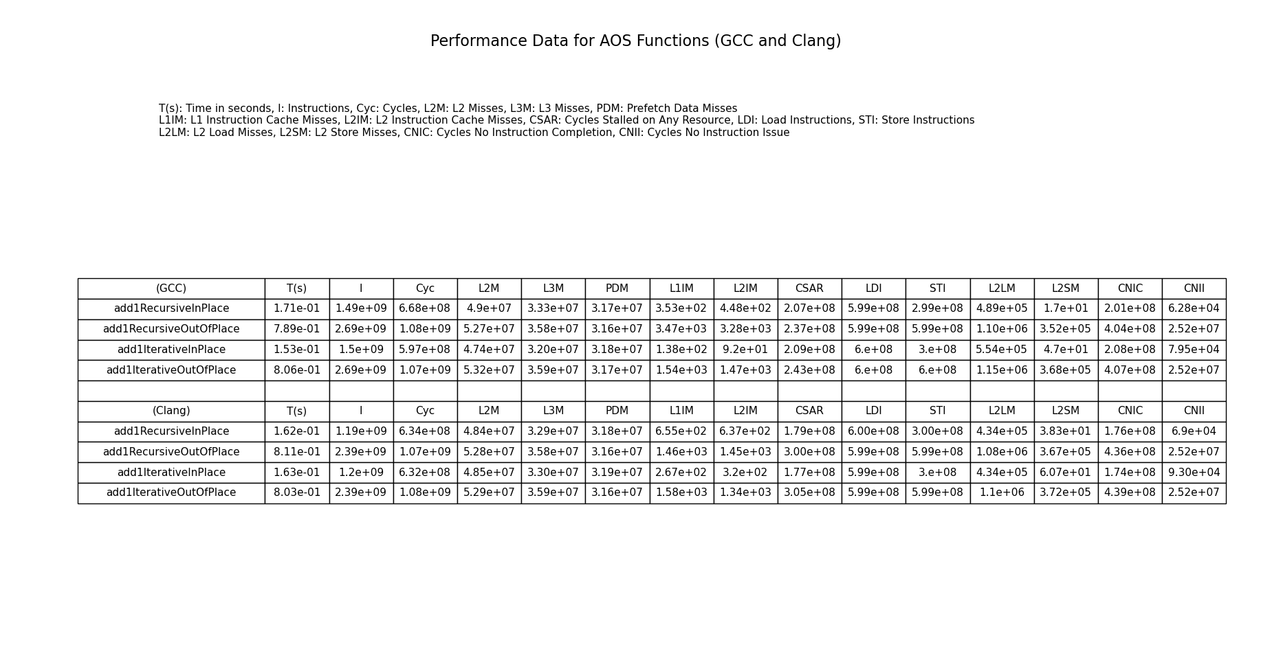
The results here are predictable. The recursive versions perform similar to the iterative versions. This is because the compiler can do a good job at tail call optimizing the tail recursive call and they are in the correct structural form.
The in place versions are faster than their out of place versions. They have fewer total instructions and take lesser cycles. The in place versions also show lower L2 and L3 cache misses. The out of place versions have more store instructions. This is because the out of place versions have to copy unused data to the output buffer. In this 1 field Cons list example, we still have to copy the data constructors in the output buffer which increases the store instructions which can be seen in the table. In addition, we have to bump the cursor for the output buffer as well. This will add more arithmetic instructions. We can also see that the L2 load and store misses have increased in the out of place versions.
The following table shows the performance figures of all the functions in the SoA representation.
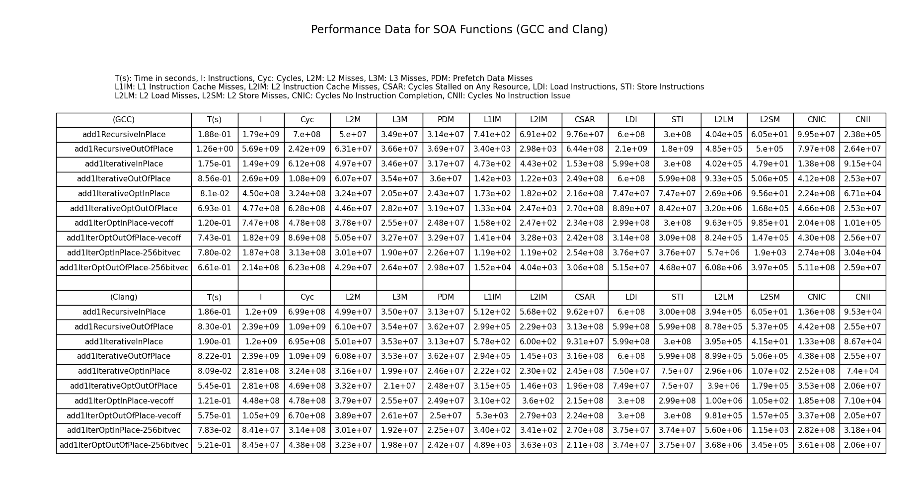
The first thing to notice is that Clang is mostly better than GCC at generating fewer instructions and getting a lower runtime. This may be because clang is doing a better job at instruction scheduling. Most of the results are predictable, the performance of the Recursive and iterative versions are similar thanks to tail call optimization. However, for add1RecursiveOutOfPlace GCC generates in-efficient code compared to the iterative version whereas Clang’s performance is similar to the iterative version. The optimized add1 in place versions are faster than the non optimized ones. They have much fewer instructions thanks to vectorization. All the versions were compiled with O3. However, for the optimized version of add1, we have a standalone O3 version, a version that switches vectorization off and another version that uses 8 lane vectorization. Note that O3 does a 4 lane vectorization by default. The fastest performance for add1 is from the in place optimized version that uses 8 lane vectorization. This is because it does not have to copy extra data and traverses lesser data. It also utilizes more vector lanes which increases efficiency. The for loop allows efficient vectorization. The iterative versions that use a while loop utilize vectorization but it is less aggressive than the for loop version.
Now focusing on the one big outlier in this table. The performance of add1RecursiveOutOfPlace for the GCC version. Its runtime is more than Clang. It generates more instructions and takes more cycles to complete. A closer look at the assembly reveals that GCC schedules the instructions differently than clang. Since x86 assembly instructions are CISC instructions, the scheduling difference may mean that the microop may have to generate more instructions for the GCC version. The difference in instruction scheduling seems to have increased the number of load and store instructions compared to clang by almost 3x. This means that Clang’s instruction scheduling may lead to a better memory optimization which requires fewer loads and stores. The CNIC (cycles no instruction was completed) is also twice for GCC which suggests that the code generated by GCC may be having more pipeline stalls due to the scheduling choices. Although, the assembly code looks mostly similar there are some minor differences in instructions and layout. The GCC code uses add instead of inc in Clang. It also uses a different jump instruction. This may have an impact on locality and pipe-lining. Since the microop is a blackbox it is hard to tell what instructions were actually executed.
The following is the Clang generated assembly for add1RecursiveOutOfPlace
0000000000001770 add1RecursiveOutOfPlace:
    1770:	48 89 d0             	mov    %rdx,%rax
    1773:	66 66 66 66 2e 0f 1f 	data16 data16 data16 cs nopw 0x0(%rax,%rax,1)
    177a:	84 00 00 00 00 00
    1780:	48 8b 0f             	mov    (%rdi),%rcx
    1783:	0f b6 11             	movzbl (%rcx),%edx
    1786:	48 ff c1             	inc    %rcx
    1789:	48 89 0f             	mov    %rcx,(%rdi)
    178c:	48 8b 0e             	mov    (%rsi),%rcx
    178f:	88 11                	mov    %dl,(%rcx)
    1791:	48 ff 06             	incq   (%rsi)
    1794:	80 fa 30             	cmp    $0x30,%dl
    1797:	75 20                	jne    17b9 add1RecursiveOutOfPlace+0x49
    1799:	48 8b 4f 08          	mov    0x8(%rdi),%rcx
    179d:	8b 11                	mov    (%rcx),%edx
    179f:	48 83 c1 04          	add    $0x4,%rcx
    17a3:	48 89 4f 08          	mov    %rcx,0x8(%rdi)
    17a7:	ff c2                	inc    %edx
    17a9:	48 8b 4e 08          	mov    0x8(%rsi),%rcx
    17ad:	89 11                	mov    %edx,(%rcx)
    17af:	48 83 c1 04          	add    $0x4,%rcx
    17b3:	48 89 4e 08          	mov    %rcx,0x8(%rsi)
    17b7:	eb c7                	jmp    1780 add1RecursiveOutOfPlace+0x10
    17b9:	c3                   	ret
    17ba:	66 0f 1f 44 00 00    	nopw   0x0(%rax,%rax,1)
The following is the GCC generated assembly for add1RecursiveOutOfPlace
0000000000401b70 add1RecursiveOutOfPlace:
  401b70:	48 89 d0             	mov    %rdx,%rax
  401b73:	48 8b 0f             	mov    (%rdi),%rcx
  401b76:	0f b6 11             	movzbl (%rcx),%edx
  401b79:	48 83 c1 01          	add    $0x1,%rcx
  401b7d:	48 89 0f             	mov    %rcx,(%rdi)
  401b80:	48 8b 0e             	mov    (%rsi),%rcx
  401b83:	88 11                	mov    %dl,(%rcx)
  401b85:	48 83 06 01          	addq   $0x1,(%rsi)
  401b89:	80 fa 30             	cmp    $0x30,%dl
  401b8c:	74 02                	je     401b90 add1RecursiveOutOfPlace+0x20
  401b8e:	c3                   	ret
  401b8f:	90                   	nop
  401b90:	48 8b 57 08          	mov    0x8(%rdi),%rdx
  401b94:	8b 0a                	mov    (%rdx),%ecx
  401b96:	48 83 c2 04          	add    $0x4,%rdx
  401b9a:	48 89 57 08          	mov    %rdx,0x8(%rdi)
  401b9e:	48 8b 56 08          	mov    0x8(%rsi),%rdx
  401ba2:	83 c1 01             	add    $0x1,%ecx
  401ba5:	89 0a                	mov    %ecx,(%rdx)
  401ba7:	48 83 c2 04          	add    $0x4,%rdx
  401bab:	48 89 56 08          	mov    %rdx,0x8(%rsi)
  401baf:	eb c2                	jmp    401b73 add1RecursiveOutOfPlace+0x3
  401bb1:	66 66 2e 0f 1f 84 00 	data16 cs nopw 0x0(%rax,%rax,1)
  401bb8:	00 00 00 00
  401bbc:	0f 1f 40 00          	nopl   0x0(%rax)
When we compare the performance of AoS vs SoA we see that the same AoS versions perform better than the SoA versions. This is because AoS versions have to execute slightly lesser instructions. They exhibit lower L2 and L3 cache misses since they only have to manage 1 allocated buffer. However, we cannot generate the optimized in place version (The one using the for loop) in the AoS representation because the data constructors and integers are interleaved. This creates two problems. One is that we cannot skip unused fields and second is that we cannot do efficient vectorization. We would have to use vector gather and scatter to load and store interleaved integers. Whereas in the SoA form we can do a vector load/store which is more efficient that a vector gather/scatter. Since add1 is a lightweight traversal, in the AoS form the memory would become a bottleneck. Note that to skip fields, we have to use in place versions of the SoA layout. In the out of place versions we still have to copy the unused fields. The add1 optimized in place version exploits both these opportunities and is indeed the fastest.
The add1RecursiveOutOfPlace function is the version of the code that the Gibbon compiler currently generates in AoS form. For GCC, the same SoA version of the function sees a speedup of 0.626x. For Clang, the SoA version sees a speedup of 0.977x. Thus for clang the performance of the AoS and SoA recursive out of place versions is similar. However, ideally we would like to generate the for loop optimized version with the SoA layout. If we can automatically transform the code to look like the optimized in place version, we can expect to see a speedup figure of around 10.11x for GCC. For Clang, we can expect a speedup of 10.35x which is similar to the GCC speedup. By shifting from the AoS layout to the SoA layout and leveraging two major properties of the code—1) no dependence across iterations for add1, and 2) in-place updates that allow us to skip writing unnecessary data and decrease store instructions—we can transform our code in a way that provides approximately a 10x speedup.
Comparison of AoS vs SoA when number of unused fields increase
We noticed from the discussion before that in place updates allow us to skip writing (copying) unnecessary data. However, is that a sufficient condition to get the desired speedup? As we see from the table, the speedup of add1RecursiveInPlace over add1RecursiveOutOfPlace in AoS for GCC is 4.614x and for Clang it is 5x. But we can’t skip over ununsed data in the AoS representation. This is because all fields are in the same buffer. Thus, if we imagine a Cursor that walks over the buffer, it has to traverse the complete buffer regardless of if there are unused fields present or not present.
In the SoA representation, since we have different buffers for different fields, we can choose to only traverse the used fields and leave the unused fields untouched but only in the in place version. The out of place version still needs to do extra work – mainly copying the unused fields to the output location. We could add an indirection to the old buffer though, which is a pointer to the old region. This is what the Gibbon compiler does at the moment to avoid copying data. Note that this is slightly different than in place updates as we are still doing additional copying and carrying an output location. When we skip unused fields, the SoA version gives us a speedup of 10.6x when comparing add1IterOutInPlace-256bitvec vs add1RecursiveOutOfPlace. Twice more than what we could get in the AoS representation.
To test this hypothesis, let us conduct yet another experiment. In this experiment, I used a python script to autogenerate the C code for both AoS and SoA. The script can take some parameters. The main ones are k (The number of total fields in the List datatype.) and l (The number of fields that the add1 traversal uses). The script can take additional parameters like size of the list etc. The scripts to auto generate the code can be found here:
A k field Cons list where k = 4 would have a data type definition is haskell like the following
type k1 = Int
type k2 = Int
type k3 = Int
type k4 = Int
data List = Cons k1 k2 k3 k4 (List) | Nil
The experiment we want to run is the following. For the same size of the list listSize, we want to fix the l value and we want to vary the k value and increase it to see the performance effects of the different functions and memory layouts (AoS vs SoA) those functions use.
We expect that in the case of the SoA memory layout, the in place versions are unaffected. they remain linear as k increases. For the out of place versions, the runtime should increase as k increases due to additional copying.
For the AoS memory layout, both the in place and out of place versions should see an increase in runtime as k increases. Since we end of traversing the full buffer even though there may be unused fields.
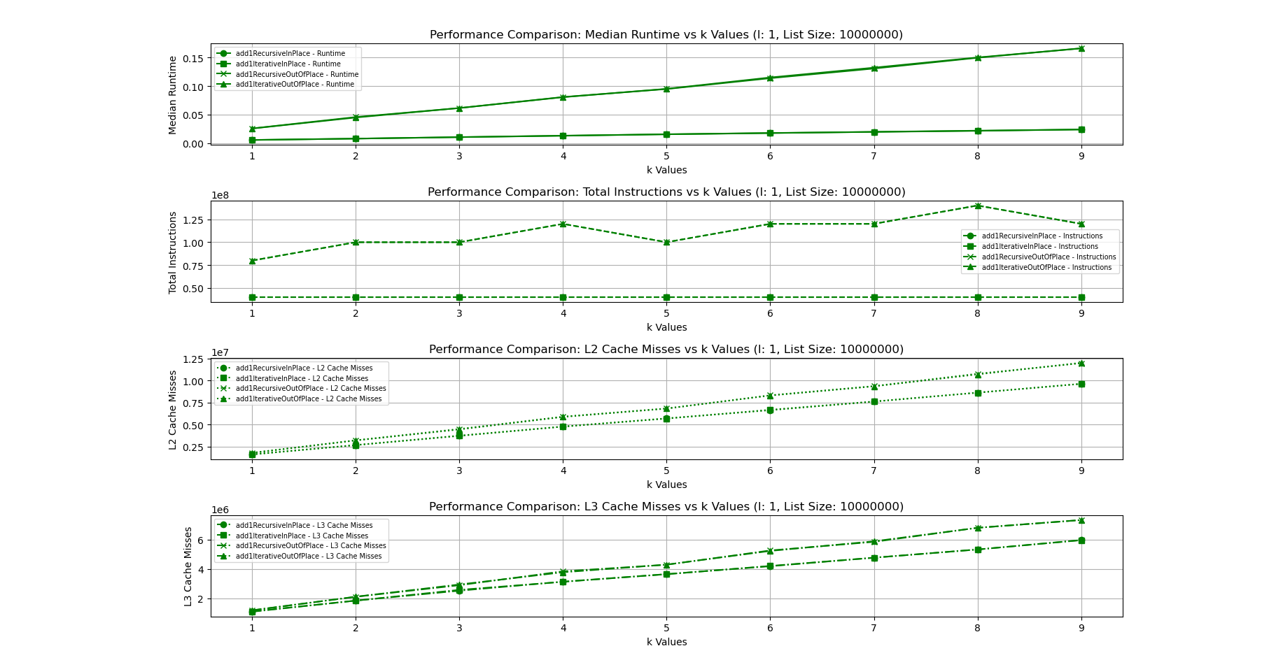
The following figure shows the runtime plotted against increasing k values when l and listSize are fixed in case of the AoS layout.
The following figure shows the runtime plotted against increasing k values when l and listSize are fixed in case of the SoA layout.
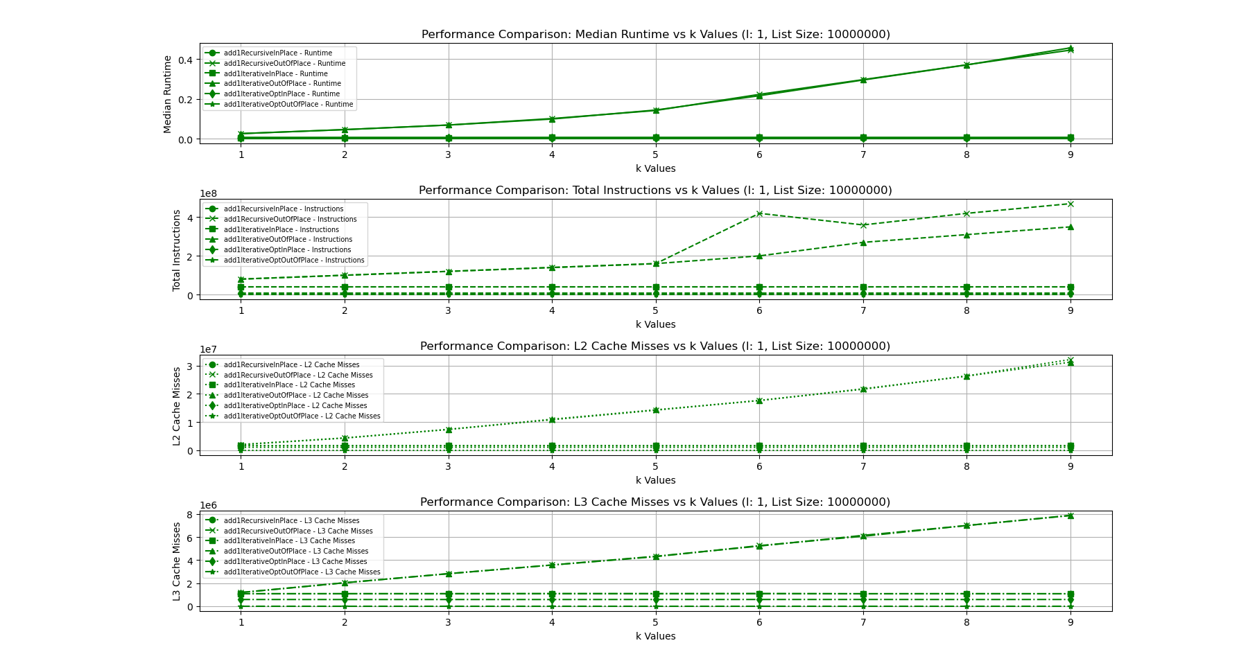
As we can see in the figures, our hypothesis is correct. In the AoS version, for all functions, the runtime increases linearly as k the number of fields in the List increases. The number of instructions is same since my code uses the first field then bumps up the cursor by numunused_fields*sizeof(field) so the number of instructions remain the same even as k increases. However, this might not always be the case. It depends on which order the fields are used in, the number of fields used among others. The L2 and L3 cache misses increase linearly as well. The basic explanation for this is fairly straightforward.
Modern x86 processors have an inbuilt prefetcher that can be enabled/disabled in the BIOS. The prefetcher loads consecutive memory addresses into the cache, with the hope that addresses that are close by will likely result in cache hits. It assumes that the program will exhibit some level of spatial locality. If we use all fields in the buffer, this is great. Since the buffer is contigously allocated, all closeby addresses in the cache will be cache hits. However as the number of unused fields increase, there will be more cache misses since nearby memory addresses will not be used as much. Thus, the cache would have to evict more data as a result. Thus, for the amount of data that the prefetcher loads into the cache, less of it is actually used. This increases both L2 and L3 cache misses.
In the SoA version, none of the in place versions are affected as k increases. The runtime remains constant. However, we see a linear increase as k increases for the out of place versions (The store operations are more in out of place versions due to additional copying). The instructions, L2 and L3 cache misses also increase as k increases for the out of place versions but they remain constant for the in place versions.
Conclusion
This case study gave us many insights. We looked at various functions that use a Cons list having two different types of memory representation. A packed AoS representation and a packed SoA representation. The SoA representation allows us to do optimizations like vectorization that can help us decrease the runtime of programs. In addition, if coupled with in place updates, the SoA representation will allow us to skip unused fields which can further decrease the runtime. This manual investigation has given us an upperbound on the performance we can expect in both cases, now, the major task would be to modify the Gibbon compiler to do this automatically for any data type definition.